
Date: 5/12/23
Convolutional Neural Network on eMNIST Dataset
Introduction
This dataset served as my introduction to the use of convolutional neural networks.
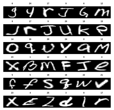
The MNIST dataset contains grey-scale, low-resolution images of hand-written letters. There are 26 categories as there are 26 letters in the alphabet, some examples are shown to the right. In this form it’s easy for us to see, but on the backend the images are structured in a way where each pixel within the image is represented as a digit between 0 and 255. The lower the digit, the darker that pixel is and vice versa.
Goal
With this dataset, the goal here is to create a model that will be able to take any of these images and correctly classify which letter it is.
Preparation
Neural networks almost always require that the input is received in a specific form. In most cases, it’s necessary to alter images such that all images are the same size etc. but the MNIST images luckily are already all have dimensions of 28 x 28. All that’s left to do is separate our dataset into 3 subsets: training data, validation data, and testing data.
Before I began using a convolutional neural network, I first created a traditional feed-forward NN. This was important because I needed something to compare my final model to. If my final model isn’t any better than a more simple NN then why bother using a convolutional NN?
Convolutional Neural Network (CNN)
In order to implement both my regular neural network and my convolutional neural network, I used the Keras API with computing power provided by Google Colab. I’ll spare the details regarding my first models, but my first NN resulted in 70% accuracy which I then improved to 85% accuracy by adding dropout. That is, my first model was able to correctly classify 70% of our test images and was improved to 81% after some improvements were made.
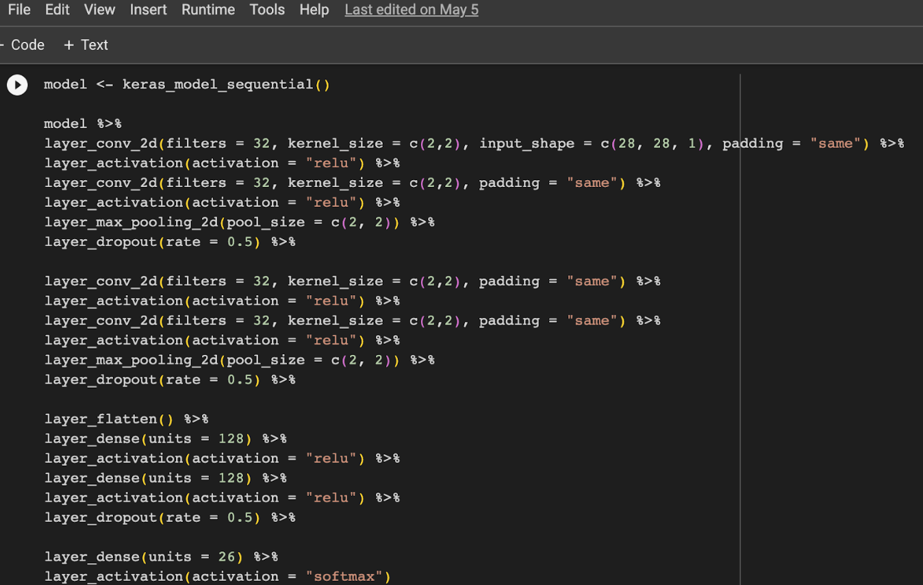
After setting my baseline, I began trying my hand at a convolutional NN. Below you’ll find the code where I structured my final convolutional NN. As you can see, this Convolutional NN was structured with many convolutional layers, max pooling layers, and activation functions. The final layer has 26 units and uses the softmax activation function. This is critical because what our model is doing is taking an image and outputting 26 different percentages, one for each letter. These percentages are interpreted as the probability that the image represents that specific letter. Our model then takes the maximum percentage and classifies the image as that letter.
Now, let’s not get ahead of ourselves. All we’ve done so far is set the structure of our model, we haven’t actually trained it! Next I compile our model, which is where I set our loss function and which metric I’d like to track (I chose accuracy)
Finally, I fit the model. On the backend, our model is classifying the images in our training dataset, getting the results of its classification, making adjustments, and repeating the process. I create the object “history” to store our loss and accuracy through each iteration of the previously mentioned process. After fitting, we can see a plot of our loss and accuracy as the training took place.
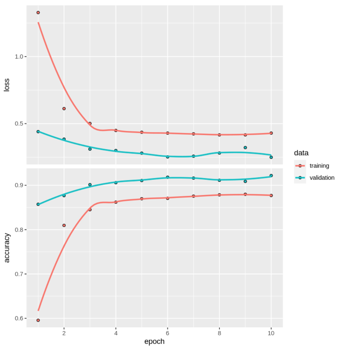
Looking at the plot, we see that the loss value and the accuracy drop and increase significantly within the first four epochs (iterations). From there, our accuracy and loss gradually improve. Finally, we have our accuracy on the CNN model. We achieved 91% accuracy!